Read Bryson and Ho Applied Optimal Control Pdf
Vivek Yadav, PhD
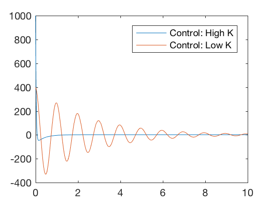
In previous classes, we saw how to use pole-placement technique to pattern controllers for regularization, ready-point tracking, tracking time-dependent signals and how to contain actuator constraints into control design. Pole-placement technique involves obtaining a gain matrix such that the resulting system dynamics under the effect of control has poles at user-specified loaction. However, we did not look into how to best choose the poles of the system. Consider the instance of a double integrator \( \ddot{x} = u \).
Consider two controllers characterized by a high and a low value of the proceeds matrix. Figures beneath illustrate that for high value of the gain matrix, the errors become to zero chop-chop, but the required control signal is very loftier. For a lower value of the gain matrix, the errors go to null much slower but the required command signal is low. Therefore, by choosing the gain matrix accordingly, a control designer can choose an optimal point betwixt the high and low gain values where the errors go to zero reasonably quickly for reasonable values of control signals. In this class, we volition visit 3 different optimal control blueprint techniques,
- Linear quadratic regulator (LQR) command formulation (showtime variance principles)
- Dynamic programming for LQR
- Path planning
- LQR using dynamic programming
- Numerical methods for optimization
- Directly collocation/Direct transcription
- Bang-blindside control
- Revisiting LQR command
clc close all clear all K_high = [ 100 40 ]; K_low = [ 40 . 8 ]; x0 = [ ten ; 0 ]; t = 0 : 0.01 : 10 ; G = K_high ; sys_fun = @ ( t , x )[ 10 ( 2 ); - Chiliad * x ]; [ t X_high ] = ode45 ( sys_fun , t , x0 ); Grand = K_low ; sys_fun = @ ( t , 10 )[ x ( 2 ); - Chiliad * 10 ]; [ t X_low ] = ode45 ( sys_fun , t , x0 ); figure ; plot ( t , K_high * X_high ',t,K_low*X_low' ) legend ( 'Control: High K' , 'Control: Low G' ) figure ; plot ( t , X_high (:, 1 ), t , X_low (:, 1 )) legend ( 'Position: High G' , 'Position: Low K' ) 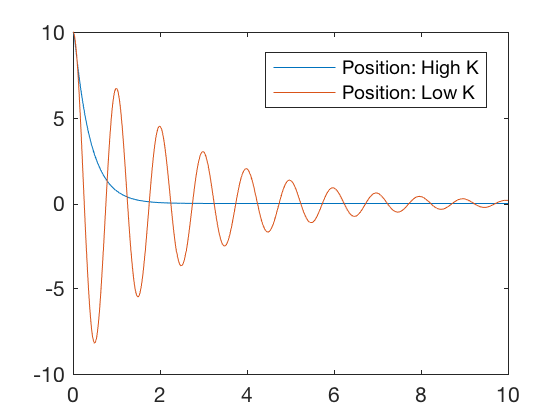
Optimal command formulation
Full general case: NO time, path or control constraint.
We start deal with the well-nigh general case of optimal control, where in that location are no constraints on the path, control signal or time to completion. Consider the system given by,
with initial status \( 10(0) = X_0 \). We wish to find a control policy \( u \) that minimizes a cost of the form,
The optimal control problem can now exist formulated as,
Subject to,
Deriving necessary weather for optimization,
The first stride in obtaining command law is to dervie the necessary conditions that the controller needs to satisfy. Nosotros exercise and then by first appending the system dynamics equation to the integrand in the error function to go,
Defining a Hamiltonian \( H( x,u,\lambda ) \) as,
The optimal control problem can now be rewritten equally,
Using integration by parts on the 2nd term in the integrant becomes
Substituting it dorsum in the integrand,
We will next takes starting time variance in \( J \) introduced by a kickoff variance \( \delta u \) in the control. Equally united states also depend on the control, a variation in command will event in variation in land, and this is represented equally \( \delta x \). Taking first variance with respect to \( u \) gives,
As \( \lambda (t) \) are arbitary, we can choose them to satisfy \( \delta J = 0 \) and for this option of \( \lambda (t) \), we get an optimal solution. The conditions for optimality can be written every bit,
with the final value condition
These equations in \( \lambda \) are as well known as costate equations. The command is given by the stationary status,
And the evolution of states is given by,
The state and co-country equation represent the necessary conditions that the optimal control law must satisfy. The boundary conditions on the state variables are defined at initial condition and the boundary atmospheric condition on co-land variables are defined at concluding time. Solving this two-betoken boundary value problem is very difficult, and several numerical methods are adult. We will look into a few of those methods later in the course. In special case where the system is linear, we can limited the costate as a linear function of states and cost equally a quadratic function of country and command, a full general state-contained solution tin be obtained.
Continuous time finite horizon, Linear quadratic regulator
For linear systems, we can get a state-independent representation of costate equation by expressing costate as a linear function of states and price is a quadratic function of state and control. This form as Linear Quadratic Control (LQR). In LQR we choose controller to minimize a quadratic cost of states and command,
Where, \( Q \) is a semi-positive definite matrix representing the cost on state deviations from 0, \( R \) is a positive-definite matrix indicating the control price, and \( S \) is a positive definite matrix penalizing the error from the final desired value of \( 0 \). \( Q \) and \( R \) are typically called equally a diagonal matrix, and college values of \( Q \) penalize trajectory error and loftier \( R \) penalizes control. Therefore, using this formulation reduces the job of command designer from identifying poles of the system, to setting relative weights of the command cost and trajectory error. The sometime is more intuitive, and a typical control design process involves varying the relative weights between trajectory errors and control costs until a satisfactory solution is obtained. Following guidelines can be used to choose satisfactory values of \( Q \) and \( R \). 'norm' is some measure of magnitude of values in the matrix, \( L_2 \) norm ( foursquare root of sum of square of all matrix entries) is a good choice.
- For \( norm(R) » norm(Q) \), command price is penalized heavily, and the resulting controller drives errors to zero slower.
- For \( norm(Q) » norm(R) \), trajectory error cost is penalized heavily, and the resulting controller drives errors to nothing very apace.
- It is possible to choose \( R \) such that the individual diagonal elements take different values. In such example, the command corresponding to larger diagonal value volition be used sparingly.
- Information technology is possible to choose \( Q \) such that the individual diagonal elements have dissimilar values. In such case, united states corresponding to larger diagonal values will be driven to zero faster.
The optimal command trouble can now be formulated as,
Discipline to,
Noting that the hamiltonian is given past,
The optimality conditions at present go,
with boundary conditions,
Nosotros expect command to be a function of states, therefore, we choose \( \lambda = P X \). Substituting,
in
and using \( \lambda = PX \) and \( \dot{X} = AX + Bu \) gives
Substituting \( u= - R^{-1}B^T \lambda = - R^{-ane}B^T PX , \)
Rearranging,
Expression above holds for all values of \(X \), therefore,
with boundary condition \( P_f = South \). The equation above is called Riccati equation, and solving it gives the optimal solution.
** Note, in this derivation nosotros causeless that the final fourth dimension is stock-still. If the final time is also a parameter that tin be varied, then an additonal condition \( \frac{\partial \Phi}{\partial t} + H_f = 0 \) is added. **
clc close all clear all t_f = 5 ; dt = 0.001 ; P_f = 100 * eye ( 2 ); Q = . 0001 * eye ( 2 ); R = ane ; A = [ 0 1 ; 0 0 ]; B = [ 0 ; i ]; P0 = P_f ; % Vectors N = t_f / dt + i ; % add t_dis array t_dis = linspace ( 0 , t_f , N ); t_res = linspace ( t_f , 0 , N ); t_dis = 0 : dt : t_f ; t_res = t_f : - dt : 0 ; P_all_res (:, length ( t_res )) = P_f (:); for i = length ( t_res ): - 1 : 2 P = reshape ( P_all_res (:, i ), size ( A )); dPdt = - ( A . '*P + P*A - P*B*B.' * P + Q ); P = P - dt * ( dPdt ); P_all_res (:, i - i ) = P (:); stop P_all_res = P_all_res ' ; X0 = [ 10 ; 0 ]; X_eul (:, 1 ) = X0 ; for i = 2 : length ( t_dis ) P_eul = reshape ( P_all_res ( i - 1 ,:), size ( A )); U_eul (:, i - 1 ) = - inv ( R ) * B '* P_eul * X_eul (:, i - one ); X_eul (:, i ) = X_eul (:, i - 1 ) + dt * ( A * X_eul (:, i - 1 ) + B * U_eul (:, i - 1 ) ); end figure plot ( t_dis ( 1 : end - 1 ), U_eul ) ylabel ( 'command' ) xlabel ( 'time' ) effigy ; plot ( t_dis , X_eul ) ylabel ( 'states' ) xlabel ( 'time' ) legend ( 'Position' , 'Velocity' ) 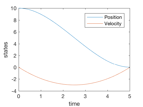
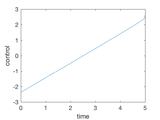
Annotation the magnitude of control bespeak is less than v units. The strategy is simple, to go downwards until half bespeak using a linearly increasing control, and and then slow down follwing the same linear command shape. None of the PID controls achieve this, farther, the required control signals in PID command is of the order of 100s.
Practical considerations
In practice, its better to save the solution of the time-dependent Riccati equation indexed by the fourth dimension to go. This way, the solution should be computed only once. For case, we can compute the vectors for P backwards for say 100 seconds. So for all controllers that crave us to be minimized within 10 seconds, the advisable P can be obtained by P corresponding to the time to get. This scheme works just for linear systems because, for linear systems \( \lambda \) is linear in states, which results in Riccati equation that is contained of current states. However, if this were not the case, and then the Riccati equation is function of states.
Continuous time infinite horizon, Linear quadratic regulator
The cost function above when time allowed to go to \( \infty \).
In steady state status, \( \dot{P} = 0 \). Therefore, the Riccati equation becomes,
The equation in a higher place is algebraic and is a quadratic matrix expression in \( P \). The solution to equation in a higher place can be obtained using MATLAB's 'care' function. Case below shows how to utilise MATLAB'southward 'care' role to calculate optimal proceeds values that minimize the toll function above.
K_high = [ 100 40 ]; K_low = [ 40 . eight ]; x0 = [ x ; 0 ]; M_a = rank ( ctrb ( A , B )); t = 0 : 0.01 : 10 ; P = care ( A , B , Q , R ); K = inv ( R ) * B '* P ; K_opt = M sys_fun = @ ( t , 10 )[ ten ( 2 ); - K_opt * x ]; [ t X_opt ] = ode45 ( sys_fun , t , x0 ); K = K_high ; sys_fun = @ ( t , x )[ x ( two ); - K_high * 10 ]; [ t X_high ] = ode45 ( sys_fun , t , x0 ); M = K_low ; sys_fun = @ ( t , ten )[ ten ( 2 ); - K_low * x ]; [ t X_low ] = ode45 ( sys_fun , t , x0 ); effigy ; plot ( t , - K_high * X_high ',t,-K_low*X_low' , t , - K_opt * X_opt ' , t_dis ( 1 : cease - 1 ), U_eul ) %legend('Control: Loftier One thousand','Command: Depression K','Control: Opt K','Position: Fixed fourth dimension') figure ; plot ( t , X_high (:, one ), t , X_low (:, 1 ), t , X_opt (:, 1 ), t_dis , X_eul ( i ,:)) legend ( 'Position: Loftier K' , 'Position: Low M' , 'Position: Opt M' , 'Position: Fixed time' ) 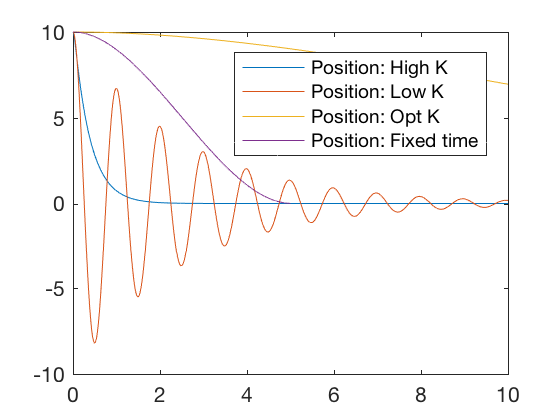
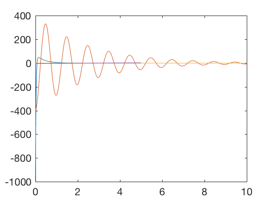
Plots higher up show that the optimal controller drives errors to zero faster and the required control bespeak is smaller. Optimal controller tin can be synthesized for discrete systems also.
Discrete time optimal control
Consider the system dynamic equation given by,
with the initial status \( X[1] = X_0 .\)
We aim to find a \( u[k] \) that minimizes,
Following a similar process as nosotros did for continuous time problems, we define a hamiltonian, \( H(10,u,\lambda ) \) as
The conditions of optimality now become,
Discrete time finite horizon, Linear quadratic regulator
Consider a linear arrangement dynamic equation given by,
with the initial status \( 10[ane] = X_0 .\)
We aim to find a \( u[k] \) that minimizes,
Following a similar process as to a higher place, it can be shown that the necessary weather for optimality are,
With boundary conditions, \( X[1] = X_0 \) and \( \lambda[Northward+1] = South X_f \).
As the equations are linear in \( X \) and \( u \), we seek a solution of the form
Using, \( 10[grand+i] = Ax[k]+ B u[k] \) and \( u[k] = - R^{-1} B^T \lambda[k+1] = - R^{-1} B^T P[yard+1] X[k+1] \) in,
gives,
Substituting in costate propogation equation gives
Equally the equation above holds for all \( 10[m] \),
Another form
Detached time equations can also be obtained in a different form, using
The costate equation is,
Rearranging gives,
As this expression holds for all \( X[thousand] \)
Detached time space horizon, Linear quadratic regulator
Consider a linear system dynamic equation given by,
with the initial condition \( X[ane] = X_0 .\)
Nosotros aim to find a \( u[thou] \) that minimizes,
Under steady state condition or space time assumption, \( P[k] = P[grand+1] \) and the Riccati equation reduces to
From the second forumation, the Riccati equation is also written as
Note, the two forms of Riccati equations are equivalent, and one follows from another via matrix inversion lemma. Link here provides a very groovy proof for matrix inversion lemma. The solution for discrete algebraic Riccati equation can be implemented in MATLAB using 'dare' command.
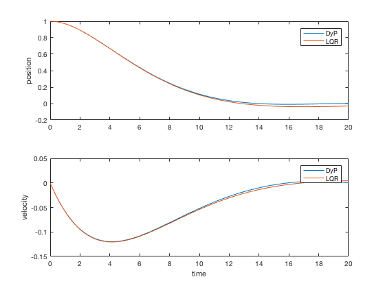
clc close all clear all t_f = twenty ; dt = 0.0001 ; t_dis = 0 : dt : t_f ; North = length ( t_dis ); S { Northward } = 100 * heart ( 2 ); R = dt ; Q = . 0001 * center ( 2 ) * dt ; A = [ 1 dt ; 0 ane ]; B = [ 0 ; dt ]; K { Northward } = [ 0 0 ]; for i = Due north - 1 : - 1 : 1 %Thousand{i} = inv(R + B'*S{i+1}*B)*B'*S{i+1}*A; %Southward{i} = Q + K{i}'*R*Grand{i} + (A-B*Grand{i})'*S{i+1}*(A-B*K{i}); % Get-go form %S{i} = Q+ A'*S{i+one}*A - A'*Southward{i+i}*B*inv(R+B'*R*B)*B'*S{i+1}*A;% 2d form S { i } = A '*inv(eye(2) + S{i+1}*B*inv(R)*B' ) * S { i + i } * A + Q ; % Third course K_norm ( i ) = norm ( Yard { i }); end X (:, 1 ) = [ 1 ; 0 ]; X_dlqr (:, 1 ) = [ ane ; 0 ]; P_dlqr = dare ( A , B , Q , R ); K_dlqr = inv ( R ) * B '* P_dlqr ; for i = 2 : N u ( i - one ) = - inv ( R ) * B '* S { i - 1 } * X (:, i - one ); X (:, i ) = A * X (:, i - ane ) + B * u ( i - 1 ); X_dlqr (:, i ) = A * X_dlqr (:, i - 1 ) - B * K_dlqr * X_dlqr (:, i - i ) ; end effigy ; subplot ( two , 1 , ane ) plot ( t_dis , 10 ( 1 ,:), t_dis , X_dlqr ( 1 ,:)) legend ( 'DyP' , 'LQR' ) ylabel ( 'position' ) subplot ( 2 , 1 , 2 ) plot ( t_dis , X ( ii ,:), t_dis , X_dlqr ( 2 ,:)) legend ( 'DyP' , 'LQR' ) ylabel ( 'velocity' ) xlabel ( 'fourth dimension' ) 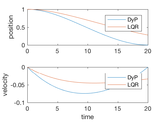
For sufficiently large time to completion, infinite-time solution and finite-time LQR give similar control signals, withal, when the final time is kept stock-still, the infinite-time approach fails. Effigy below present comparison of finite-time and space-time outputs for large concluding time. As tin can exist seen, the controller performances are equivalent in the two cases.
** Note: LQR solution using MATLAB'southward 'care' or 'cartel' commands are applicable only for infinite time problems. **
Above we derived necessary conditions that an optimal controller has to satisfy. We practical it to discrete and continuous LQR issues and saw one method of computing optimal command to drive errors to nada in a finite time. However, the method above has some limitations,
- Non all cost functions tin be expressed as LQR problem. Consider the example when we are trying to minimize the time to go.
- LQR formulations do not generalize well to conditions when additional constraints are imposed on the arrangement.
- For control inequality constraints, the solution to LQR applies with the resulting control truncated at limit values.
- Dealing with state- or state-control (mixed) constraints is more than difficult, and the resulting conditions of optimality are very complex. Run into Applied optimal control, past Bryson and Ho for detailed treatment.
In the cases in a higher place, numerical methods are more suitable.
Dynamic programming
The algebraic equations derived higher up are very difficult to solve under non-steady state (non-infitite time) assumptions. In such cases, numerical techniques tin exist used. One such technique is dynamic programming. Dynamic programming is easily applicable to discrete-time problem linear quadratic regulator trouble. Dynamic programming is a clever arroyo to solving sure types of optimization problems, and was developed by Richard Bellman. Its a very versatile method, and can exist applied to several different issues. Examples include, path planning, generating shortest cost path between cities, inventory scheduling, optimal control, rondevous problems and many more than. The master objective is to compute a cost-to-become role at each state value. Once this toll-to-get map is bachelor, the optimal command policy can be obtained by moving from one state to another state that minimizes the toll to go from that state. A general dynamic programming problem tin be represented equally,
In many cases, the expression to a higher place is modified as,
The factor \( \gamma \) discounts the future cost-to-go values. A \( \gamma = 0\) results in an algorithm that completely ignores the future cost-to-go, where as a large \( \gamma \) considers the future rewards more than. Having \( \gamma \) is as well helpful in numerical methods where we do not know the cost-to-go to beginning with and guess it recursively. Having a \( \gamma \) term reduces the contributions of early incorrect assumptions.
Therefore, the chore of solving optimal control reduces to finding the cost-to-go function. This can be accomplished by solving backwards from the desired state to all the possible initial values. Once this toll-to-go office is known, the optimal control policy reduces to finding the trajectory that minimizes cost from current state to a future state, and cost-to-go from there. Dynamic programming approach is a very generic algorithm and tin be practical to optimization problems where cost-to-go and cost of moving from 1 state to another are additive. Before getting into detailed algroithm development, lets look at a elementary case.
Simple example: Dynamic programming
Consider the problem of finding the shortest path between the target and and any start position on the grid in the figure below. We presume that we can move only left, correct, up and down, and each action costs the states 1 point.
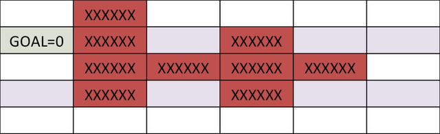
In the example to a higher place, its hard to compute optimal path starting from an initial condition. Yet, it is much easier to compute cost-to-become if we start from the goal, and stride backwards. After the first step, the cells above and below goal have a cost-to-go of 1.

We can comport on this step for next iv cycles, at which fourth dimension, the price-to-get associated with each jail cell looks as follows. Notation, the cells in a higher place and to the right of cell corresponding to 5-points both accept a score of 6.
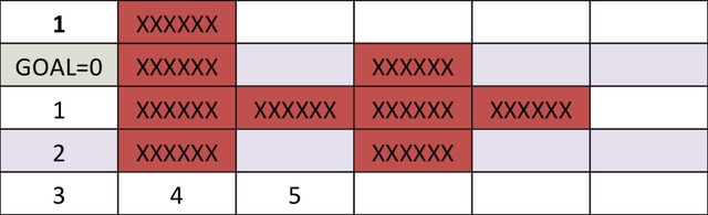
The price-to-get map for target location is,

One time nosotros have the cost-to-go for the grid-goal configuration, we can start at any point on the grid and reach the goal by following the path that minimizes the sum of action (one) and toll-to-go. The algorithm performed to a higher place is dynamic programming.
Pseudocode to programmatically implement dyanamic programming is as follows,
- Initialization
- Set cost-to-go, J to a large value.
- Discretize state-action pairs
- Set cost-to-get as 0 for the goal.
- Set point_to_check_array to incorporate goal.
- Repeat until elements in point_to_check_array = 0
- For betoken element in point_to_check_array
- Step backwards from point, and compute price of taking activity to move to the point every bit price-to-go from point plus the activeness cost.
- If current cost-to-go, J is larger than the cost-to-go from betoken to moved country, then update price-to-go for the moved state.
- Add moved state to a new point_to_check_array
- For betoken element in point_to_check_array
In do, the algorithm above is difficult to implement, a simpler but computationally more than expensive algorithm is as follows,
- Initialization
- Set up toll-to-get, J to a large value.
- Discretize state-action pairs
- Fix cost-to-go as 0 for the goal.
- Set point_to_check_array to contain goal.
- Repeat until no-values are updated,
- For each chemical element in the filigree, accept all the possible actions and compute the incurred costs.
- For each action, compute the toll-to-go of the new state.
- Update self if cost-to-get of the new land plus action is lower than current toll-to-become.
Below is result of applying the algorithm above to
Dynamic programming: Path-planning
Consider the task of obtaining the shortest path between a desired and concluding position, given the configuration of obstacles in the environment. We tin can apply a like technique as higher up.
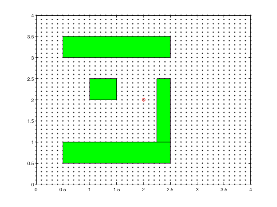
The cost-to-get evolves as shown in the blitheness below. Every bit tin be seen, all the regions corresponding to the obstacles are very high values, and regions closer to the target have lower values.
Dynamic programming in control vs reinforcement learning.
The aforementioned ideas of dynamic programming can exist applied in reinforcement learning also. However, in reinforcement learning the objective is to maximize reward, and in control theory objective is to minimize cost. Below is algorithm for using reinforcement learning that maximizes the reward.
Dynamic programming for linear quadratic regulator control
We volition next apply the procedure to a higher place to compute optimal control for a linear system given by,
Consider designing a controller for the
with
being the price at the end of the cycle. Nosotros offset the dynamic programming by stepping backwards from \( N \)
As
Therefore,
Note that \( x[N-1] \) does not depend on \( u[N-1] \), therefore, optimal price-to-become can be computed by taking derivatives with respect to \( u[North-1] \), using matrix derivatives,
Equally \( R \) and \( S_N \) are symmetric,
We can rewrite the command above every bit \( u[N-i] = - K_{N-1} X[North-1] \) where,
The cost function \( J(10[N-ane]) \) can at present be written as,
If nosotros write \( J(x[N-1] ) \) as \( \frac{1}{2} X[N-one]^T S_{Northward-1} Ten[N-i]\), and then
The expression above is the Riccati equation we got before with \( Southward \) substituted for \( P \). The toll-to-go expression between \( ( Due north-2) \) and \( ( N-one) \) is now,
with
Dynamic programming for continuous systems involves discretizing the cost-to-become past computing price between one interval and next every bit the integral of the cost of control (integrand).
Dynamic programming: LQR instance
Consider the system given by \( \ddot{ten} = u \), we wish to find a control that minimizes
with the final state condition to minimize,
Nosotros convert this chore into dynamic programming chore past discetizing the system as,
Corresponding parameters for cost-to-get at present become, \( S_N = 10I\), \( Q = 0 \) and \( R = dt \). Nosotros volition use the equations below to recursively calculate \( S_N southward \) and so integrate states forward to compute the optimal command. In practice, \( Q = 0 \) gives numerically unstable results, and then we use \( Q = 0.001 dt I \).
clc shut all clear all t_f = iv ; dt = 0.02 ; t_dis = 0 : dt : t_f ; Due north = length ( t_dis ); S { N } = 100 * eye ( 2 ); R = dt ; Q = . 0001 * eye ( two ) * dt ; A = [ one dt ; 0 1 ]; B = [ 0 ; dt ]; K { N } = [ 0 0 ]; K_norm ( N ) = 0 ; for i = N - 1 : - 1 : 1 Yard { i } = inv ( R + B '*S{i+1}*B)*B' * Due south { i + 1 } * A ; Due south { i } = Q + K { i } '*R*K{i} + (A-B*Chiliad{i})' * Due south { i + 1 } * ( A - B * Yard { i }); K_norm ( i ) = norm ( K { i }); end X (:, 1 ) = [ ane ; 0 ]; X_dlqr (:, 1 ) = [ one ; 0 ]; P_dlqr = cartel ( A , B , Q , R ); K_dlqr = inv ( R ) * B '* P_dlqr ; for i = 1 : N - 1 u ( i ) = - K { i } * X (:, i ); Ten (:, i + 1 ) = A * Ten (:, i ) + B * u ( i ); X_dlqr (:, i + i ) = A * X_dlqr (:, i ) - B * K_dlqr * X_dlqr (:, i ) ; end figure ; subplot ( two , 1 , 1 ) plot ( t_dis , X ( one ,:), t_dis , X_dlqr ( 1 ,:)) fable ( 'DyP' , 'LQR' ) ylabel ( 'position' ) subplot ( two , ane , 2 ) plot ( t_dis , Ten ( 2 ,:), t_dis , X_dlqr ( two ,:)) legend ( 'DyP' , 'LQR' ) ylabel ( 'velocity' ) xlabel ( 'time' ) 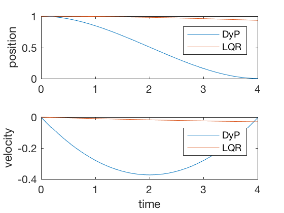
** Notation: Hamilton Jacobi Bellman equation is the continuous-time analog of dynamic programming for discrete systems. The atmospheric condition for optimality can be obtained using this equation too. **
Numerical methods for optimal control: Shooting methods
In most control applications, there are many constraints, such every bit actuators cannot apply infinite control, actuators dynamics, the physical limits on states of the system, and further as control designers we could make up one's mind to introduce additional contraints. The optimization criteria tin exist expressed every bit,
Problem formulation, optimal control with constraints
Find control sequence to minimize,
Subject to,
with initial condition \( X(0) = X_0 \), under constraints,
where \( C_{eq} \) and \( C \) are equality and inequality constraints on state and control variables.
For control inequality constraints, the solution to LQR applies with the resulting control truncated at limit values. However, dealing with land- or state-control (mixed) constraints is more than difficult, and the resulting weather condition of optimality are very circuitous. Several numerical techniques have been developed to design optimal control for such problems. Nosotros will try to solve this problem using numerical methods. In item, we volition work with ane set up of methods called multiple shooting and direct collocation.
There is likewise a set of indirect collocation methods, where we derive the necessary weather for optimal control, and make sure the polynomial approximations satisfy the necessary conditions for optimality at the collocation points. This method is typically more than accruate, but is not generalizable to different types of problems, considering the necessary conditions are very problem specific.
Shooting methods
Weather of optimality are divers every bit 2 point boundary value problems where the states are defined in the initial status, and costate variables are defined in the final position. Typical solution process involves guessing some value of control sequences to kickoff with, integrating the states fowrard, applying the last land constraints and integrating the costate and state equation backwards. The resulting initial value is compared to the starting initial value, and the control sequence is updated to reduce this error. This process is called unmarried shooting. Shooting comes from the idea of integrating us forrad using a numerical technique, such equally euler integration or runge-kutta 4 integration. Integrating forrard and astern usually results in large errors because whatever errors in control policy'due south assumptions propogates through out the system. Ane fashion to avoid these errors is to utilize multiple shooting where nosotros discretize the entire trajectory into smaller grids, and we assume the command and state policies in each interval to be polynomials. These points are called knot points. Every bit the command and land variables are arbitary polynomials, they practise non satisfy the dynamic equations. Therefore, dynamic equations are introduced as constraints at some intermediate points. In virtually methods, we cull these points and knot points as the aforementioned. Notwithstanding, this results in more variables to be optimized. Further, if we have information regarding control variables, say for example, we wait command to be a cubic function, we tin can utilize this information to inform our optimizer. Case below illustrates the idea of multiple shooting.
Parametarization of optimial control using polynomial functions
Limited states and command as a piece-wise continuous role of time,
The control is parametrized by knot points, \( u_i \) and \( q_i \) for \( i \) going from \( 1 to N+ane \).
Find control sequence to minimize,
Subject field to,
with initial status
with command
under constraints,
The cost part above is now a parameter optimization problem in knot points. Nonlinear programming techniques can exist used to solve such problems. Numerical optimization methods are approximate methods, and involve a lot of 'fine-tuning'. This procedure is best illustrated by an example.
Nonlinear programming: quick review
As state to a higher place, we convert optimal command problem into a simpler task of identifying the knot-points, coefficient of polynomials or other parameters that define a state/control trajectory. This is a parameter optimization problem, and is much simpler than solving LQR equations. Say nosotros want to minimize \( f(Ten) \), such that,
Such issues can be solved using nonlinear solvers, such as fmincon.
Fmincon: example 1
Bailiwick to the constraint that,
fun = @ ( x ) 100 * ( ten ( ii ) - x ( 1 ) ^ 2 ) ^ two + ( i - x ( 1 )) ^ 2 ; x0 = [ 0.5 , 0 ]; A = [ 1 , 2 ]; b = 1 ; Aeq = [ 2 , 1 ]; beq = 1 ; x = fmincon ( fun , x0 , A , b , Aeq , beq ) Fmincon: Canon case
Consider the instance of firing a cannon such that the cannonball reaches a item target while requiring minimum firing energy. The equations of motion describing the movement of cannon ball are given by,
The objective of optimization is given by,
The boundary weather condition are given by,
clc close all clear all N_grid = 10 ; t_f = 3 ; v_x = four ; v_y = 10 ; X0 = [ t_f ; v_x ; v_y ]; X_opt = fmincon ( @ ( X ) cost_fun_cannon ( X ), X0 ,[],[],[],[],[],[], @ ( X ) cons_fun_cannon ( Ten ), options ); %%% Constraint part function [ C , Ceq ] = cons_fun_cannon ( X ) N_grid = ( length ( 10 ) - 3 )/ 3 ; t_f = X ( i ); vx = 10 ( 2 ); vy = Ten ( 3 ); d_x = t_f * vx ; d_y = vy * t_f - i / 2 * 9.8 * t_f ^ two ; C = [ - t_f + 0.001 ; - vx ; - vy ]; Ceq = [ d_y - 10 ; d_x - ten ; ]; %%% Cost part function toll = cost_fun_cannon ( Ten ) N_grid = ( length ( Ten ) - 3 )/ 3 ; % Price fun t_f = X ( 1 ); vx = X ( two ); vy = X ( 3 ); cost = vx ^ 2 + vy ^ 2 ; 
Bang-bang command
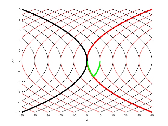
Lets consider the a example of designing control for a double integrator whose control tin can vary between -1 and 1. If we want to reach from some starting bespeak say 0 to 10, the fastest control solution is to employ 1 control for one-half the fourth dimension, and then use -1. This control tin besides be indicated by a phase-plot between position and velocity. The red lines point trajectory for the instance when command is i, and black lines indicate trajectories when control is -i. The states motility on contour lines in clockwise directions. The least-time cost for a particle starting at 0 to go to 10 is given by the green line.
Problem formulation,
Given the double integrator organization \( \ddot{X} = u \),
given,
Solution
Nosotros describe control as a piece-wise constant part, and the position and velocity variables defined at the knot points form the additional input to the optimizer. Nosotros then integrate the states starting with ane knot point to some other bold this control and apply equality constraints betwixt this and the next point. The lawmaking snippet below shows this. Consummate MATLAB code unlike examples can be found here.
role [ C , Ceq ] = cons_fun_doubleIntegrator ( X , blazon ) % Bold cosntant U N_grid = ( length ( 10 ) - 1 )/ 3 ; % Cost fun t_f = 10 ( 1 ); X1 = X ( 2 : N_grid + 1 ); X2 = X ( 2 + N_grid : 2 * N_grid + 1 ); u = 10 ( 2 + 2 * N_grid : 3 * N_grid + 1 ); C = []; Ceq = [ X2 ( 1 ) - 0 ; X2 ( end ) + 0 ; X1 ( one ); X1 ( finish ) - x ; ]; time_points = ( 0 : 1 /( N_grid - 1 ): i ) * t_f ; for i = ane :( N_grid - ane ) X_0 ( 1 ,:) = X1 ( i ); X_0 ( 2 ,:) = X2 ( i ); t_start = time_points ( i ); t_end = time_points ( i + ane ); tt = t_start :( t_end - t_start )/ 10 : t_end ; [ t , sol_int ] = ode45 ( @ ( t , y ) sys_dyn_doubleIntegrator ( t , y , X , type ), tt , X_0 ); X_end = sol_int ( terminate ,:); Ceq = [ Ceq ; X_end ( one ) - X1 ( i + ane ); X_end ( 2 ) - X2 ( i + 1 )]; % IMPOSING DYNAMIC CONSTRAINTS AT BOUNDARIES. end 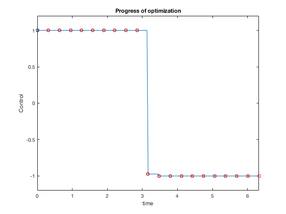
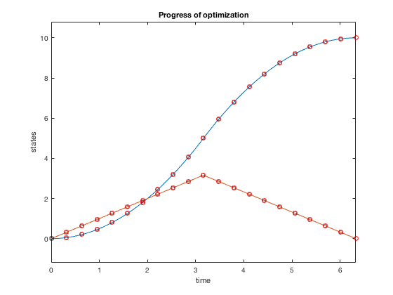
Plots above nowadays results from optimization. The optimal command strategy that minimizes fourth dimension of motility while obeying control constraints is one where you accelerate using maximum control, and decelerate using maximum control.
Bang-bang control: Example 2
At present we impose additional constraint that the velocity cannot go to a higher place ane.v. The problem changes as, given the double integrator organization \( \ddot{X} = u \),
given,
Calculation additional constraints in Multiple shooting framework is easy. Nosotros express the optimization problem equally before, however, add additional constraint, that velocity at knot points must be less than 1.5. This tin can exist incorporated by adding just 1 line of code.
role [ C , Ceq ] = cons_fun_doubleIntegrator ( X , type ) % Assuming cosntant U N_grid = ( length ( X ) - 1 )/ three ; % Price fun t_f = X ( 1 ); X1 = X ( two : N_grid + one ); X2 = X ( 2 + N_grid : 2 * N_grid + 1 ); u = X ( 2 + 2 * N_grid : three * N_grid + i ); C = []; function [ C , Ceq ] = cons_fun_doubleIntegrator ( X , blazon ) % Assuming cosntant U N_grid = ( length ( Ten ) - ane )/ three ; % Cost fun t_f = X ( 1 ); X1 = X ( ii : N_grid + 1 ); X2 = X ( 2 + N_grid : ii * N_grid + 1 ); u = 10 ( ii + two * N_grid : 3 * N_grid + one ); C = [ X2 - i.5 ]; % IMPOSING VELOCITY CONSTRAINT. Ceq = [ X2 ( i ) - 0 ; X2 ( cease ) + 0 ; X1 ( 1 ); X1 ( end ) - 10 ; ]; time_points = ( 0 : 1 /( N_grid - 1 ): 1 ) * t_f ; for i = ane :( N_grid - 1 ) X_0 ( 1 ,:) = X1 ( i ); X_0 ( 2 ,:) = X2 ( i ); t_start = time_points ( i ); t_end = time_points ( i + i ); tt = t_start :( t_end - t_start )/ ten : t_end ; [ t , sol_int ] = ode45 ( @ ( t , y ) sys_dyn_doubleIntegrator ( t , y , X , type ), tt , X_0 ); X_end = sol_int ( stop ,:); Ceq = [ Ceq ; X_end ( 1 ) - X1 ( i + 1 ); X_end ( 2 ) - X2 ( i + 1 )]; % IMPOSING DYNAMIC CONSTRAINTS AT BOUNDARIES. stop 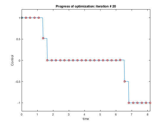
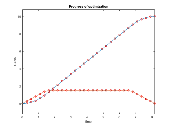
Plots above bear witness how control policy and states evolve for the the case when velocity is constrained to be less than one.v. The controller accelerates the particle to the velocity limit using maximum control, so maintains that velocity for some time, and decelerates using maximum decelerating control.
Below are some applied guidelines for desgining optimization routines,
- Initialization is very crucial. Its good to initialize states and velocities as linear functions, and control as 0.
- The resulting command policy satisfies constraints and dynamic equations only at the knot points. Therefore, to ensure condom have a safe margin within the limits, and so intermediate points exercise not violate boundary constraints.
- In cases where you know the course of control equation (polynomial, piecewise abiding), use information technology to inform the optimizer.
- Optimality (lowest cost solution) tin can be improved by either changing the number of grid points or club of polynomials. However, systems with more parameters accept larger
- Beginning with a simpler depression-dimensional polynomial on a coarser grid and apply this to inform an optimizer with more parameters.
Conclusion
In this lesson nosotros went over some concepts of optimal control. Nosotros saw how to develop optimal command for linear systems, then looked into designing optimal command under land and command constraints using multiple shooting method. Multiple shooting has one disadvantage that nosotros demand to define velocity and position both, which results in \(2 N_{grid} \times N_{position}\) variables. Withal, we did non impose any strict conditions on the state variables. If we approximated postion variables by shine polynomials whose derivatives are equal at knot points, then the velocity variables are derivative of position variables, and i set of dynamic constraints are satisfied. Therefore, only boosted constraint left to satisfy is the second social club condition relating acceleration to position and velocity variables. This technique is called direct collocation, which we will discuss in the adjacent class.
hillyerinctiary1996.blogspot.com
Source: https://mec560sbu.github.io/2016/09/25/Opt_control/
Belum ada Komentar untuk "Read Bryson and Ho Applied Optimal Control Pdf"
Posting Komentar